
グラフ作成に必要なパッケージをインストールします。
- phyloseq ―― 構成要素のデータを組み立てるために必要
- ggplot2 ―― グラフ作成に必要
# phyloseqとggplot2をインストールする。
installed.packages("phyloseq")
installed.packages("ggplot2")

#パッケージの呼び出し
library("phyloseq")
library("ggplot2")
ggplot2のテーマを指定する。
theme_set() を用いてggplot2 のテーマを指定することで、好みのデザインのグラフを作ることができます。 theme_gray()やtheme_bw()、theme_dark()、theme_light()、theme_linedraw()、theme_minimal()などがあります。
今回は、theme_set(theme_bw())にしてみます。
theme_set(theme_minimal())今回は練習で、仮のOTUデータセットを作成します。
otumat = matrix(sample(1:100, 100, replace = TRUE), nrow = 10, ncol = 10)
outmatというオブジェクトに、1から100までの数字からサンプリングした数字の、縦10行×横10行のデータセットを作成する。
- matrix() ―― 行列の作成
- sample() ―― ランダムにサンプリング(標本を抽出)する
   otumat = matrix(sample(1:100, 100, replace = TRUE), nrow = 10, ncol = 10)
   otumat
         [,1] [,2] [,3] [,4] [,5] [,6] [,7] [,8] [,9] [,10]
    [1,]   83   81   50   45   31   84   65   21   60    70
    [2,]   61   31    3   82   79    5   79   39   99    83
    [3,]   27   40   93   48   27   55   33   73   17    73
    [4,]   83   39   40   35   81   85   12   60   52    60
    [5,]   51   65   64   32   56   42   32   66   51    45
    [6,]   41   96   91   79   33   26   85   78   42    66
    [7,]    6    6   62   20   19   32   55   72  100    54
    [8,]   14   59    8   80   35   61   86   25   84    88
    [9,]    3    5    9   48   77   62   16   22   16    55
   [10,]   74   13   27   44   46   21    7   41   25    20
ランダムサンプリングなので、実行ごとに数字が変わります。
   otumat = matrix(sample(1:100, 100, replace = TRUE), nrow = 10, ncol = 10)
   otumat
         [,1] [,2] [,3] [,4] [,5] [,6] [,7] [,8] [,9] [,10]
    [1,]   57   45   84   97    5   65    7   62   87    99
    [2,]   60   73   40   48   14    3   25   18   46    51
    [3,]   71   96   69   29   45   42   86   93   71    43
    [4,]    2   38    8   73   37   63   93   51   94    66
    [5,]   59   69   14    5   45    8   74    2   45    21
    [6,]   85   91   83    1   41   54   12   75   79    35
    [7,]   77   64   97   62   12   69   61   74   57    35
    [8,]   58  100   38   86   16   84   37   45   39    68
    [9,]   54   46   28   90   46   33   99   23   73    67
   [10,]    7   99   68   64   14   77    1   42   78    17
行と列に名前を付けます。
   rownames(otumat) <- paste0("OTU", 1:nrow(otumat)) #列に名前を付ける
   colnames(otumat) <- paste0("Sample", 1:ncol(otumat)) #行に名前を付ける
   otumat
         Sample1 Sample2 Sample3 Sample4 Sample5 Sample6 Sample7 Sample8 Sample9 Sample10
   OTU1       57      45      84      97       5      65       7      62      87       99
   OTU2       60      73      40      48      14       3      25      18      46       51
   OTU3       71      96      69      29      45      42      86      93      71       43
   OTU4        2      38       8      73      37      63      93      51      94       66
   OTU5       59      69      14       5      45       8      74       2      45       21
   OTU6       85      91      83       1      41      54      12      75      79       35
   OTU7       77      64      97      62      12      69      61      74      57       35
   OTU8       58     100      38      86      16      84      37      45      39       68
   OTU9       54      46      28      90      46      33      99      23      73       67
   OTU10       7      99      68      64      14      77       1      42      78       17
paste0() ―― ()の中の要素に文字列を加えて、つなげる。
さっきまで1,2,3,4…だった縦の列に、”OTU”の文字列が加わりました。
行の列には、”Sample”の文字列が加わりました。
仮の分類表のデータも作成します。
taxmat = matrix(sample(letters, 70, replace = TRUE), nrow = nrow(otumat), ncol = 7)
 rownames(taxmat) <- rownames(otumat)
 colnames(taxmat) <- c("Domain", "Phylum", "Class", "Order", "Family", "Genus", "Species")
 taxmat

  Domain Phylum Class Order Family Genus Species OTU1  "u"    "o"    "n"   "e"   "q"    "w"   "a"
 OTU2  "j"    "z"    "h"   "b"   "d"    "w"   "n"
 OTU3  "a"    "d"    "v"   "m"   "n"    "a"   "c"
 OTU4  "y"    "h"    "i"   "f"   "z"    "s"   "v"
 OTU5  "i"    "n"    "l"   "t"   "a"    "o"   "r"
 OTU6  "l"    "q"    "c"   "g"   "g"    "q"   "i"
 OTU7  "c"    "s"    "g"   "v"   "z"    "w"   "h"
 OTU8  "u"    "f"    "s"   "b"   "n"    "q"   "g"
 OTU9  "j"    "u"    "y"   "w"   "d"    "h"   "o"
 OTU10 "i"    "q"    "d"   "e"   "q"    "r"   "d"
otu_table ―― OTUの豊富さのオブジェクトの構築
tax_table ―― 分類名の表を作成する
   library("phyloseq")
   OTU = otu_table(otumat, taxa_are_rows = TRUE)
   TAX = tax_table(taxmat)
   OTU
   OTU Table:          [10 taxa and 10 samples] #10分類と10サンプル
                        taxa are rows
         Sample1 Sample2 Sample3 Sample4 Sample5 Sample6 Sample7 Sample8 Sample9 Sample10
   OTU1       57      45      84      97       5      65       7      62      87       99
   OTU2       60      73      40      48      14       3      25      18      46       51
   OTU3       71      96      69      29      45      42      86      93      71       43
   OTU4        2      38       8      73      37      63      93      51      94       66
   OTU5       59      69      14       5      45       8      74       2      45       21
   OTU6       85      91      83       1      41      54      12      75      79       35
   OTU7       77      64      97      62      12      69      61      74      57       35
   OTU8       58     100      38      86      16      84      37      45      39       68
   OTU9       54      46      28      90      46      33      99      23      73       67
   OTU10       7      99      68      64      14      77       1      42      78       17
physeq = phyloseq(OTU, TAX)
physeqphyloseq() ―― 構築メソッドの一つ。構成データから得られる実験レベルオブジェクトを作成できる。
グラフを出力します。
plot_bar(physeq, fill = "Family")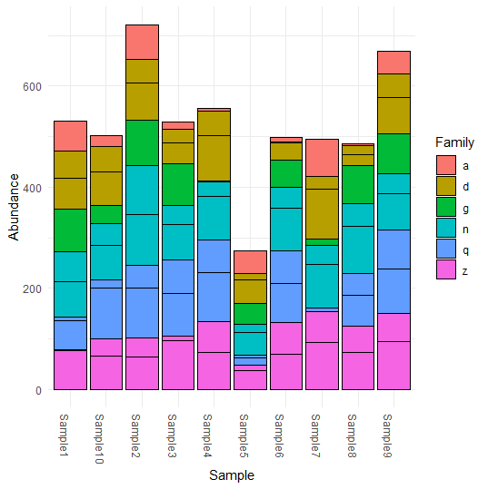
参考:http://joey711.github.io/phyloseq/import-data
こんにちは。
大学で土壌中の真菌について研究しているものです
phyloseqとggplotsをCRANからインストールしたときのRのバージョンを教えていただきたいです。
こんにちは。ご質問ありがとうございます。
ggplot2は3.3.6、phyloseqは1.38.1だったかと思います。
ご返信ありがとうございます。
質問が分かりにくく申し訳ありません。
パッケージをインストールした時の’R自体’のバージョンです。
お手数をお掛けしますが、よろしくお願い致します。
大変失礼しました。4.1.1だったと思うのですが、記憶が曖昧です。
すみません…。
ご返信ありがとうございます!
いえいえ!研究頑張ってください。